Introduction
In this lab, we are becoming acquainted with the simulation environment, a Python-based software platform that provides a virtual map and a virtual robot. The robot can be controlled either through a Python program or manually using the keyboard. It supplies various data for analysis, including front-facing distance sensor readings, odometry readings, and the ground truth of the robot's location. Note that the sensor readings will contain noise. The simulation environment also features a 2D plotter for visualizing odometry readings and ground truth trajectories. By the end of the lab, we will have implemented two control strategies: (a) open-loop control, where the robot travels in a square loop, and (b) closed-loop obstacle avoidance control.
Bayes's Filter
A Bayesian filter is a probabilistic framework used for estimating the state of a dynamic system over time by applying Bayes' theorem. It represents the state as a probability distribution, which is updated iteratively through two main steps: prediction and update. In the prediction step, the filter uses a motion model to forecast the next state based on the current state and control inputs, incorporating uncertainty in the process. In the update step, the filter incorporates new observations using a sensor model to adjust the predicted state distribution. This combination of prediction and update allows the Bayesian filter to handle uncertainty and noise in sensor data effectively, making it widely used in applications like robot localization, tracking, and sensor fusion.
Localization
Bayesian filtering plays a crucial role in localization algorithms, particularly in probabilistic approaches such as Monte Carlo Localization (MCL) or the Extended Kalman Filter (EKF). Here's how Bayesian filtering is connected with localization:
- State Estimation: In localization, the robot's state typically includes its position and orientation (pose) in the environment. Bayesian filtering allows us to represent this state as a probability distribution, capturing the uncertainty associated with the robot's pose.
- Prediction Step: The robot predicts its next pose based on its motion model and control inputs (e.g., velocity commands). Bayesian filtering enables the prediction of the next state while considering uncertainty in the motion model and control inputs. This prediction yields a probability distribution of the robot's potential future poses.
- Update Step: When the robot receives sensor measurements (e.g., from a GPS receiver, visual odometry, or range sensors), Bayesian filtering updates the predicted pose distribution using Bayes' theorem. The likelihood of each possible pose given the sensor data is calculated using a sensor model, incorporating noise and uncertainty in the sensor readings. The resulting updated pose distribution reflects the most probable locations of the robot given the sensor measurements.
- Iterative Process: Localization with Bayesian filtering is an iterative process. After each prediction and update step, the robot's pose distribution is refined, providing a progressively more accurate estimate of its true pose over time.
Sensor Model
The sensor model, assumed to follow a Gaussian distribution of noise, represents the inaccuracies and uncertainties inherent in sensor measurements. In practice, real-world sensors such as lidar, cameras, or range finders often produce noisy data due to environmental factors, sensor limitations, and interference. The Gaussian distribution is a common choice for modeling sensor noise, as it accurately captures the random variations in sensor readings around their true values.
Motion Model
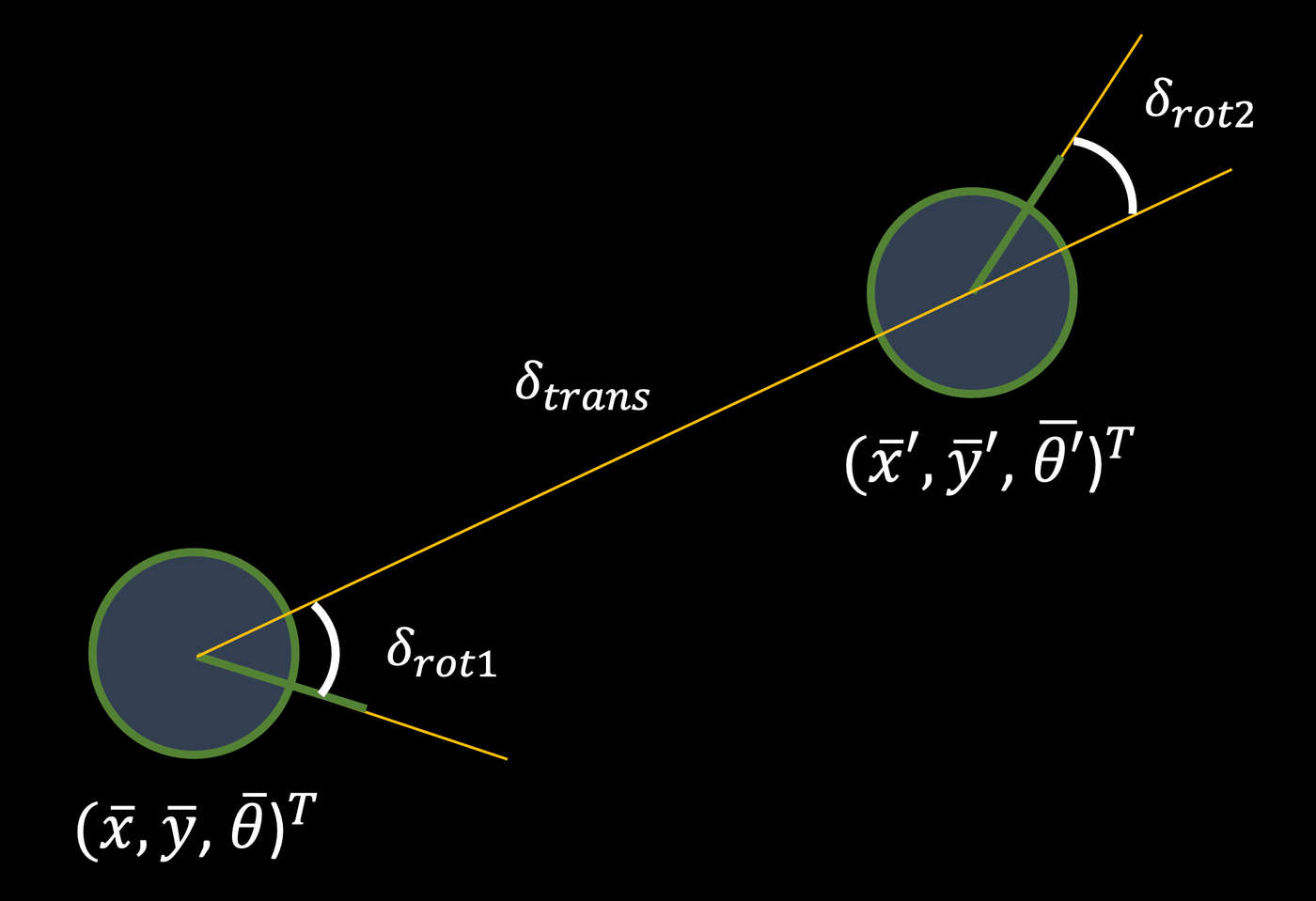
The odometry motion model characterizes the robot's movement between successive poses based on control inputs, such as wheel encoder readings or motor commands. It breaks down the movement into three components: initial rotation, translation, and final rotation. The initial rotation accounts for any change in orientation at the beginning of the movement, while the translation represents the linear displacement of the robot. Finally, the final rotation accounts for any additional change in orientation at the end of the movement. By incorporating these components, the odometry model provides a systematic way to estimate the robot's movement, allowing for accurate localization and navigation in the environment.
Algorithms
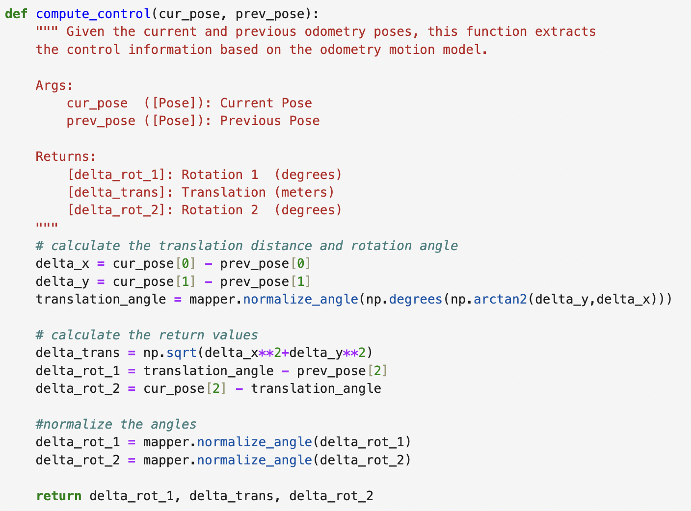
Compute Control
The compute_control() function accepts the current pose and the previous pose as inputs. By analyzing the difference between these poses, it calculates the components necessary to characterize the robot's movement according to the odometry model. These components include the initial rotation, translation, and final rotation, which collectively represent the steps involved in estimating the robot's motion between consecutive poses.
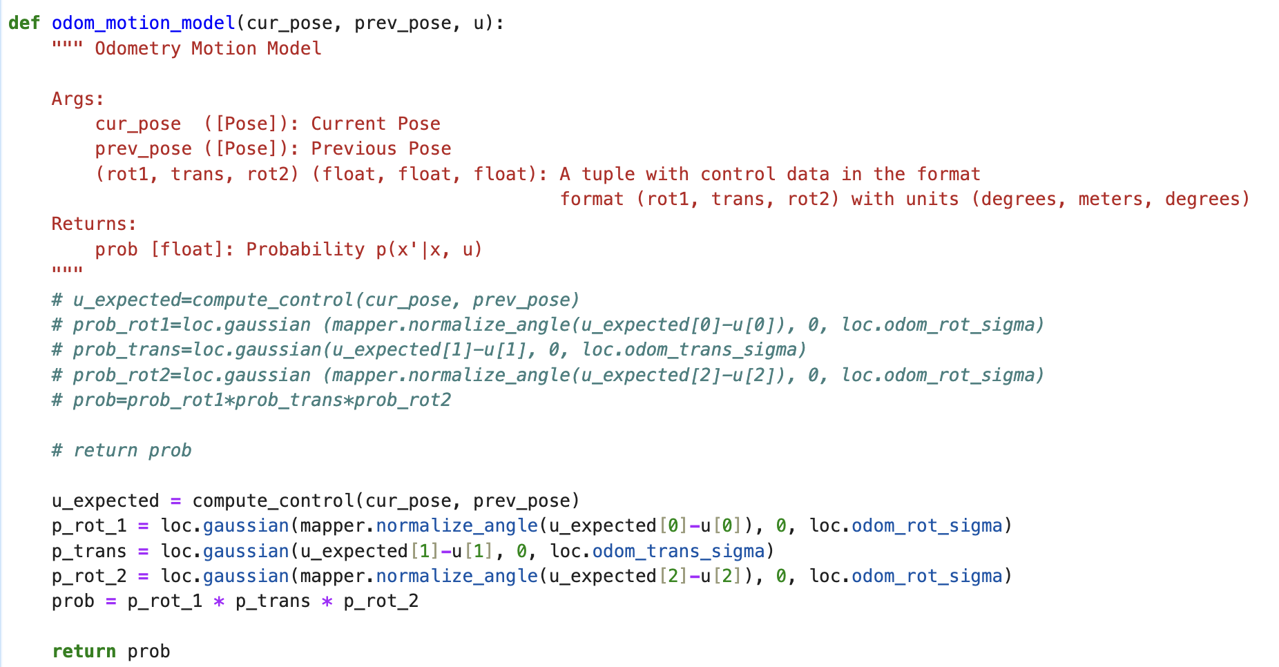
Odometry Motion Model
The odom_motion_model() function operates by receiving a current pose and a previous pose as inputs. It then utilizes the compute_control() function to extract the odometry model parameters from these poses. Subsequently, the function calculates the probabilities associated with these parameters, treating them as Gaussian distributions. These distributions are centered on the control input u and have standard deviations provided as relevant parameters. This process ensures that the motion model accounts for uncertainty by modeling the variability in the odometry model parameters.
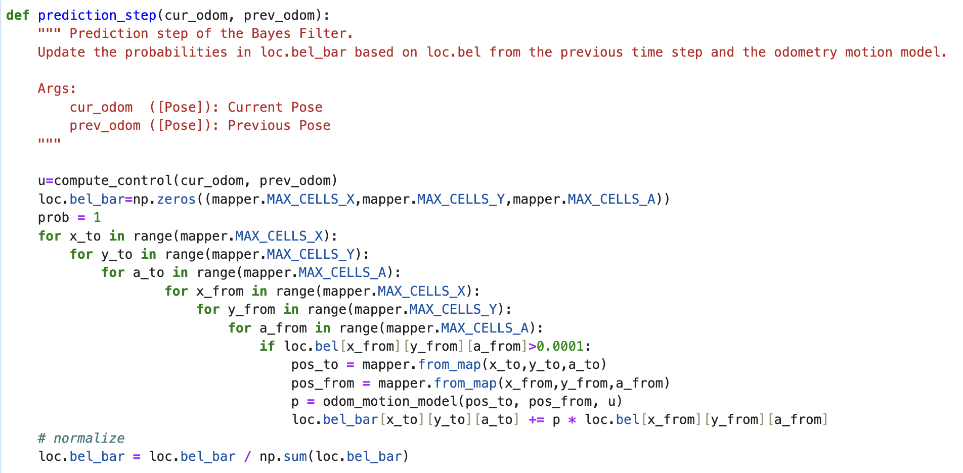
Prediction Step
The prediction_step() function operates by taking a current and previous odometry state as inputs. It then extracts the odometry model parameters from these states and iterates over the entire grid of discretized cells for both the previous and current poses. During this process, it constructs a predicted belief using the odom_motion_model() function. For each cell, the probabilities calculated by the motion model are multiplied together and tallied for the entire grid. Finally, the probabilities are normalized to form a distribution summing to 1. Given the substantial computational requirements associated with covering the 3D simulation volume, an optimization strategy is implemented. This involves disregarding probabilities smaller than 0.0001, as they make negligible contributions to the belief. While this approach reduces computational complexity, it comes at the expense of filter accuracy.
Sensor Model
The sensor_model() function operates by accepting an array of observations as input. It calculates the probabilities of each observation occurring for the current state, treating them as Gaussian distributions with a provided standard deviation. This process enables the assessment of the likelihood of each observation given the current state, facilitating the update of the belief state in the Bayesian filtering framework.

Update Step
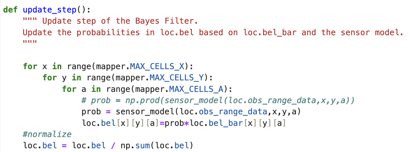
The update_step() function iterates over the grid for the current state and retrieves the sensor model data using the sensor_model() function. It then utilizes this data to update the belief state. The updated belief represents the robot's estimation of its position in the discretized environment based on the sensor observations. Finally, the belief is normalized to ensure that the probabilities sum to 1, providing a coherent representation of the robot's estimated position.
Simulation
The initial video illustrates a trajectory and localization simulation lacking a Bayes filter. In this visualization, the deterministic odometry model is depicted in red, contrasting with the ground truth trajectory tracked by the simulator, which is displayed in green. As the simulation progresses, it becomes evident that the odometry model, operating independently, yields poor results. The trajectory portrayed by the odometry model extends beyond the map's boundaries, demonstrating erratic behavior and failing to align with the expected path.
In the subsequent video, the integration of a Bayes filter into the localization simulation is demonstrated. Despite the inadequacy of the direct odometry model, indicated by the trajectory in red, the introduction of a probabilistic belief, visualized in blue, yields a significantly improved approximation of the robot's true position. Notably, the probabilistic approach excels in proximity to walls, where sensor data is more reliable and consistent, resulting in a more accurate localization. Conversely, its efficacy diminishes in open spaces, such as the center of the map, where sensor data may be less reliable.